I’ve decided to make a very simple temperature logger using the BeagleBone black and a readily available and Texas Instrument’s LM74 temperature sensor. The sensor is not the most precise one out there but it is easy to interface to and costs under $2. LM74 communicates over SPI, a popular and well supported interface. To hook up the sensor only 5 wires are needed:
BeagleBone Black to LM74

BB signal
BB Header_Pin
SPI signal
 LM74 signal
 LM74 pin


SPI0_d1
P9_18
Master Data Out
 N/A
 N/A


SPI0_d0
P9_21
Master Data In
SI/O
 1


SPI0_SCLK
P9_22
Clock
SC
2


SPI0_CS
P9_17
Chip Select
CS
7


GND
P9_1
N/A
GND
4


3.3V
P9_3
N/A
V+
8

Since we don’t care about sending data to the sensor, only reading data back, the SPI Data Input line of the beagle bone is left unconnected.
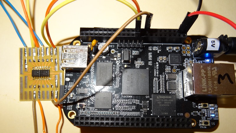
Here is a picture of my setup. I’ve put two temperature sensor on the same perf-board just because I had space and to do some more testing later.
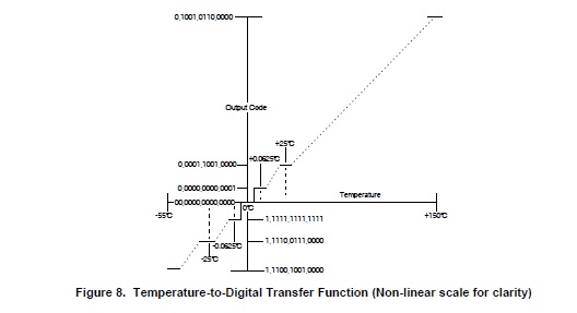
 According to the datasheet all we need to do to get data out of this guy is to power it with 3 to 5.5v volts, set the chip select low and send 16 clock pulses (2 bytes). LM74 will transmit 16bits of data (only 13 of which actually contain useful info but more on that later)
I’ve chosen to write my data logging application in Python since there are tons of libraries and support available for it.
Overall goal is to read the SPI data, convert it to a meaningful temperature value and write to a file along with a time stamp.
Here is the full code:
# ========= IMPORTS =============
import os
import sys
from time import sleep
from Adafruit_BBIO.SPI import SPI
import logging

# =========== Initialization Scripts =============
print "Server _ON_"
print "Open SPI"
spi = SPI(0,0) #(bus, device)
spi.mode=0 #[CPOL][CPHA] values from 0..3
spi.msh=2000000
spi.open(0,0)
APP_ROOT = os.path.dirname(os.path.realpath(sys.argv[0])) #gets current directory where script resides

def twos_comp(val, bits):
 #compute the 2's compliment of int value val
 if (val & (1 << (bits - 1))) != 0: # if sign bit is set e.g., 8bit: 128-255
 val = val - (1 << bits) # compute negative value
 return val # return positive value as is

def spi_read_LM74():
 #read SPI data from LM74 sensor
 #clock - P9_22
 #data out - P9_18 (not connected)
 #data in - P9_21
 #chip select - P9_17
 global spi #use the globally defined "spi", prevents from having to open/close spi on every read
 read_val_list=spi.xfer2([0,0]) #clock out two bytes of pulses. Read data in. Data out is not connected.
 #print(format(read_val_list[0], '#010b'),format(read_val_list[1], '#010b'))
 read_val=(read_val_list[0] << 8) | read_val_list[1] # concatenate into a single 16bit value
 read_val = (read_val >> 3) & 0x1FFF #only 13 upper bits of data are temperature data
 read_val = twos_comp(read_val,13)
 temperature = read_val * 0.0625;
 print "Temp = ", temperature
 return temperature

def main():
  #logging.basicConfig(format='%(asctime)s;%(message)s', filename=APP_ROOT+'/temp.log', level=logging.INFO)
 logging.basicConfig(format='%(asctime)s;%(message)s',
       datefmt='%Y-%m-%dT%H:%M:%SZ', #UTC format for easier use in Java Script
       filename=APP_ROOT+'/temp.log',
       level=logging.INFO)
 while(1):
 logging.info(spi_read_LM74()) #read temperature value and write to log file
 sleep(1) #sleep for one second
 pass

if __name__ == '__main__':
 main()
At initialization Adafruit’s SPI library automatically loads the “ADAFRUIT-SPI0” cape (the library needs to be installed beforehand). “main” function first configures logging and then enters a forever loop that reads the LM74 data and writes it to a file. Python’s logging library is very useful, alternatively I could have written the data to a file of my choosing manually. Benefits of using is that it creates the log file for you if it doesn’t already exist, adds the time stamp and there are ways of limiting the size of the file (not implemented in this code).
Reading the SPI data is done in the “spi_read_LM74” function. First we transmit two dummy bytes [0,0] just to generate 16 clock pulses. As prevsiously mentioned the Master Out Slave In (MOSI) line is not even connected. At the same time the slave (LM74) transmits its 16 bits of data back to the beagle bone. Note that the Chip Select (CS) line must stay low for the entire 16bit transmission, that’s why spi.xfer2 function is used. This data is captured in the “read_val_list” variable as a list of two bytes. read_val_list[0] is the first byte received and contains the higher 8 bits, read_val_list[1] contains the lower 8 bits. Per LM74’s datasheet bits 15:3 contain temperature data encoded as two’s compliment value with one LSB = 0.0625 °C. So we first concatenate the two 8 bit values, then bit-wise shift to the right and mask with 0x1FFF. At this point we have the 13 bits of data but since it is in two’s complement format we need to “decode it” using the “twos_comp” function. The function returns a signed integer which is the temperature data we need just scaled by 0.0625. Last step is to multiply by this value and the result is a floating point decimal value in °C
Logging function takes care of adding this data to a file and the process starts all over again. The resulting temp.log is a simple text file that contains date&time “;” temperature and looks something like:
2015-02-18 04:16:27,100;24.75
2015-02-18 04:16:28,105;25.0625
2015-02-18 04:16:29,111;25.0625
2015-02-18 04:16:30,117;24.6875
2015-02-18 04:16:31,122;24.4375
2015-02-18 04:16:32,132;24.3125
2015-02-18 04:16:33,137;24.1875
2015-02-18 04:16:34,143;24.0625
2015-02-18 04:16:35,149;24.0625
2015-02-18 04:16:36,154;24.0
2015-02-18 04:16:37,165;23.875
2015-02-18 04:16:38,171;23.8125
2015-02-18 04:16:39,177;23.75
2015-02-18 04:16:40,183;23.75
2015-02-18 04:16:41,188;23.6875
2015-02-18 04:16:42,197;23.75
Of course staring at a text file is not very exciting. The next step is to add a CherryPy server and display a dynamic temperature chart. Stay tuned.
Entire project is located at this BitBucket Git repository.